
Recently, we have presented a paper titled: Bayesian analysis of fracture of polyamide 12 U-notched specimens, in collaboration with the group of Professor Jesús Rodríguez-Pérez (DIMME, Grupo de Durabilidad e Integridad Mecánica de Materiales Estructurales, Escuela Superior de Ciencias Experimentales y Tecnología, Universidad Rey Juan Carlos) in the European Conference of Fracture 2024
We share the Python code in this blog using synthetic notched fracture data as an example of Bayesian non-linear regression.

We describe step by step the code used
import numpy as np
import matplotlib.pyplot as plt

import pymc as pm
import arviz as az
def KN_func(KIC, ft, R):
pi = np.pi
L = (KIC / ft) ** 2 * 1000
KN = KIC * (1 + pi * R / L) ** 1.5 / (1 + 2 * pi * R / L)
return KN
# Fixed parameters for synthetic data
KIC = 3.25
ft = 82.0
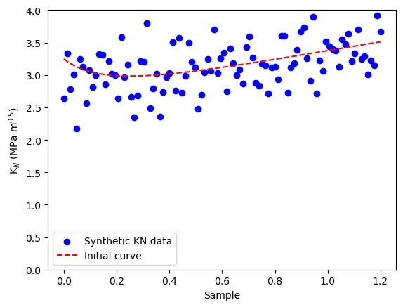
# Generate synthetic data
N = 100 # Number of data points
radio_vect = np.linspace(0, 1.2, N)
mean_KN = KN_func(KIC,ft, radio_vect)
# Adding noise to simulate real measurements
observed_KN_values = mean_KN + np.random.normal(0, 0.3,N)
# Plot the synthetic data
plt.scatter(radio_vect, observed_KN_values, color='blue', label='Synthetic KN data')
plt.plot(radio_vect,mean_KN, color='red', linestyle='--', label='True KN curve')
plt.xlabel('Sample')
plt.ylabel(r'K$_N$ (MPa m$^{0.5}$)')
plt.ylim([0,None])
plt.legend()
plt.show()
- KIC: Represents the critical stress intensity factor (fracture toughness).
- ft: Critical stress.
- ϵ: The error parameter.
We’ll specify priors for the two material parameters, and, the standard deviation.
with pm.Model() as model:
    # Priors for KIC, ft, and R based on domain knowledge
    KIC = pm.Uniform('KIC', 1, 5)
    ft = pm.Uniform('ft', 10, 150)
    ϵ = pm.InverseGamma('ϵ', alpha=1.0,beta=1)

    # Likelihood: observed data is compared against the model function
    KN_observed = pm.Normal('KN_observed', mu=KN_func(KIC, ft, radio_vect), sigma=ϵ, observed=observed_KN_values)

    # Inference
    trace = pm.sample(2000, tune=1000, return_inferencedata=True,cores=3)
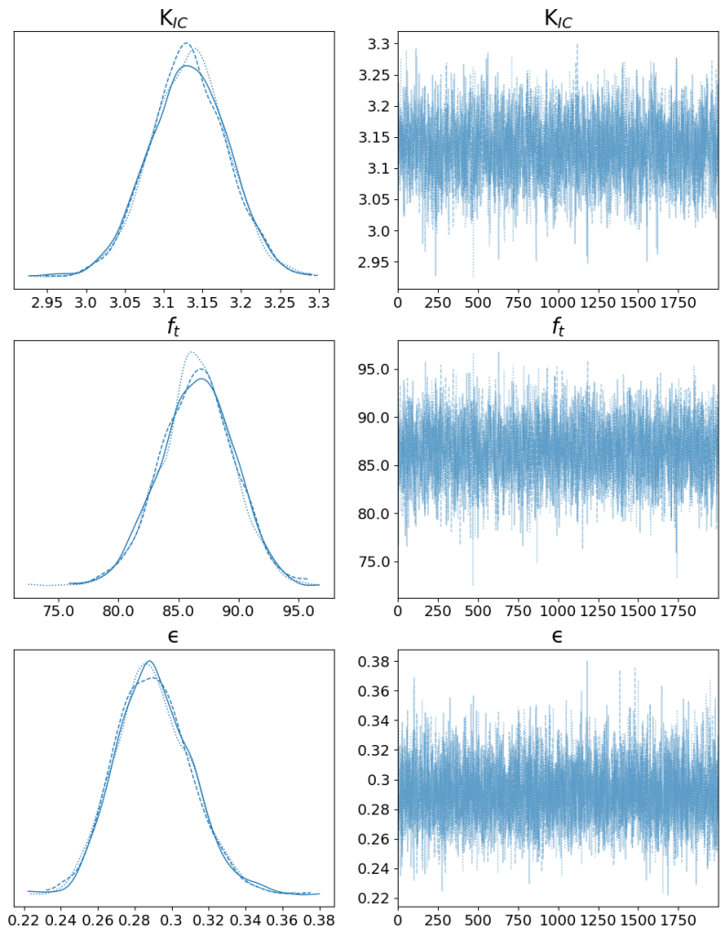
Using arviz, a powerful library for Bayesian analysis, we plot the trace of the parameters and their posterior distributions:
trace_fig = az.plot_trace(trace, var_names=[ 'KIC', 'ft','ϵ'], figsize=(12, 15));

# get and change x labels
for i in range(trace_fig.shape[0]):
    for j in range(trace_fig.shape[1]):
        if j==0:
            x_labels = [str(np.round(x,3)) for x in trace_fig[i][j].get_xticks()];
            trace_fig[i][j].set_xticklabels(x_labels, fontsize=14);

        if j==1:
            y_labels = [str(np.round(y,3)) for y in trace_fig[i][j].get_yticks()];
            trace_fig[i][j].set_yticklabels(y_labels, fontsize=14);

            x_labels = [str(int(x)) for x in trace_fig[i][j].get_xticks()];
            trace_fig[i][j].set_xticklabels(x_labels, fontsize=14);

        title=trace_fig[i][j].get_title()
        trace_fig[i][j].set_title(title, fontsize=20);

trace_fig[0][0].set_title(r'K$_{IC}$',  fontsize=20);
trace_fig[0][1].set_title(r'K$_{IC}$',  fontsize=20);

trace_fig[1][0].set_title(r'$f_{t}$',  fontsize=20);
trace_fig[1][1].set_title(r'$f_{t}$',  fontsize=20);
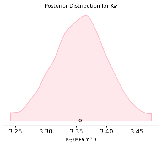
The posterior distribution can be plotted in better quality
# Plot the posterior distribution for KIC
az.plot_density(trace, var_names=['KIC'], shade=0.3, hdi_prob=0.99,colors='lightpink')
plt.xlabel(r'K$_{IC}$ (MPa m$^{0.5}$)')
plt.title('Posterior Distribution for K$_{IC}$')
plt.show()
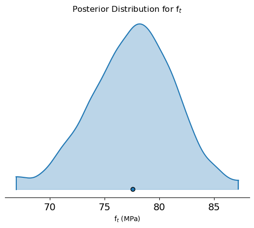
az.plot_density(trace, var_names=['ft'], shade=0.3, hdi_prob=0.99)
plt.xlabel(r'f$_{t}$ (MPa)')
plt.title('Posterior Distribution for f$_{t}$')
plt.show()
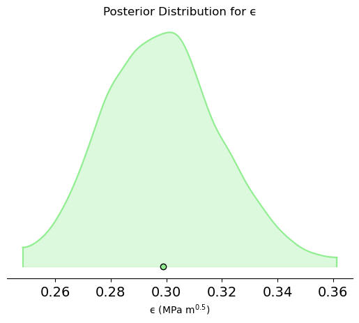
az.plot_density(trace, var_names=['ϵ'], shade=0.3, hdi_prob=0.99,colors='lightgreen')
plt.xlabel(r'ϵ (MPa m$^{0.5}$)')
plt.title('Posterior Distribution for ϵ')
plt.show()
# Summarize the results
summary = az.summary(trace)
print(summary)
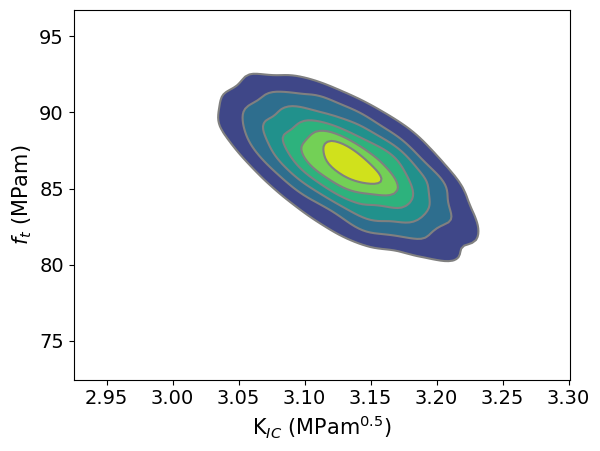
The parameter region that fits the experimental results can be studied with the next code
az.plot_pair(trace,kind='kde', var_names=[ 'KIC', 'ft'])
plt.ylabel(r'$\sigma_{C}$ (MPam)')
plt.xlabel(r'K$_{IC}$ (MPam$^{0.5}$)')
# Posterior samples
posterior_KIC = trace.posterior['KIC'].values.flatten()
posterior_ft = trace.posterior['ft'].values.flatten()

KICmean = trace.posterior['KIC'].mean().values
ftmean = trace.posterior['ft'].mean().values
fit_KN = KN_func(KICmean,ftmean, radio_vect)

# Select some posterior samples for plotting
num_samples = 500  # Number of samples to plot
posterior_samples_idx = np.random.choice(len(posterior_KIC), num_samples, replace=False)

# Plot original data vs. posterior curves
plt.scatter(radio_vect, observed_KN_values, color='blue', label='Observed KN data')
for i in posterior_samples_idx:
    plt.plot(radio_vect, KN_func(posterior_KIC[i], posterior_ft[i], radio_vect), color='gray', alpha=0.1)

# Plot the true KN curve
plt.plot(radio_vect, fit_KN, 'r--', label='Fitted curve', linewidth=2)
plt.xlabel('Sample')
plt.ylabel(r'K$_N$ (MPa m$^{0.5}$)')
plt.ylim([0,None])
plt.legend()
plt.show()
