Programming a Bayesian Statistical Fit in Python for Linear Regression

Bayesian statistical fitting is a powerful technique for data analysis that allows us to incorporate prior information and update it with observed evidence. In this blog, we’ll explain how to perform a Bayesian fit for linear regression using Python, with the goal of estimating the model parameters while quantifying uncertainty.

This tutorial describes step by step how to perform a Bayesian Statistical fit for Linear Regression

Step 1: Installing PyMC3 and Required Libraries

First, install necessary libraries

pip install pymc3 numpy matplotlib seaborn

Step 2: Importing the Libraries

Import the required libraries

import numpy as np
import matplotlib.pyplot as plt
import seaborn as sns
import pymc3 as pm

Step 3: Synthetic Data

Let’s create a synthetic dataset that follows a linear relationship with some added noise:

# Generate data
np.random.seed(42)
n_samples = 200
X = np.linspace(0, 10, n_samples)
true_intercept = 1.0
true_slope = 2.5
noise = np.random.normal(0, 1, n_samples)

# Observed data
Y = true_intercept + true_slope * X + noise

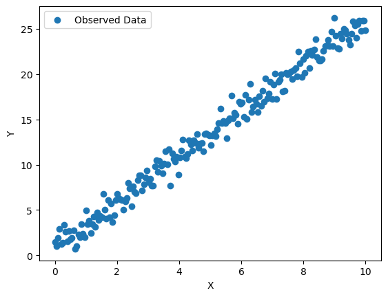
# Plot the data
plt.scatter(X, Y, label='Observed Data')
plt.xlabel('X')
plt.ylabel('Y')
plt.legend()
plt.show()

Step 4: Bayesian Model

The Bayesian model for linear regression is defined using PyMC3. The prior distributions enclose the regression parameters (intercept and slope) and the noise standard deviation.

# Define the Bayesian model
with pm.Model() as bayesian_model:
    # Priors for the parameters
    intercept = pm.Normal('intercept', mu=0, sigma=10)
    slope = pm.Normal('slope', mu=0, sigma=10)
    sigma = pm.HalfNormal('sigma', sigma=1)

    # Linear regression model
    mu = intercept + slope * X

    # Likelihood
    Y_obs = pm.Normal('Y_obs', mu=mu, sigma=sigma, observed=Y)

    # Inference
    trace = pm.sample(1000, tune=1000, cores=2, target_accept=0.95)

In this model:

Priors are initial assumptions about the parameters, specified as normal distributions in this case.

Likelihood models the relationship between the observed data and the model parameters.

Step 5: Analyzing the Results

Let’s analyze the results and visualize the posterior distribution of the estimated parameters.

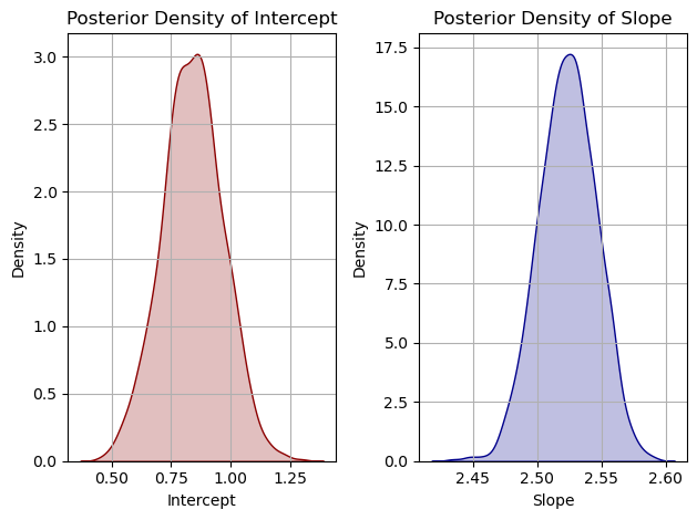
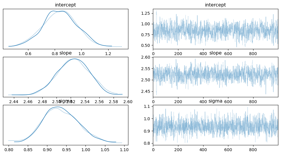
# Summary of the results
pm.summary(trace)

# Plot the posterior distributions
pm.traceplot(trace)
plt.show()

Step 6: Visualizing the Bayesian Fit

Visualize the Bayesian linear regression fit compared to the observed data.

# Generate posterior predictive samples
with bayesian_model:
    posterior_pred = pm.sample_posterior_predictive(trace, var_names=['intercept', 'slope'], samples=100)

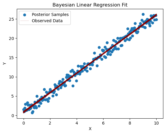
# Plot the predictions
plt.scatter(X, Y, label='Observed Data')
for i in range(100):
    pred_y = posterior_pred['intercept'][i] + posterior_pred['slope'][i] * X
    plt.plot(X, pred_y, color='darkred', alpha=0.1)
plt.xlabel('X')
plt.ylabel('Y')
plt.title('Bayesian Linear Regression Fit')
plt.legend(['Posterior Samples', 'Observed Data'])
plt.show()

Conclusion

Bayesian fitting for linear regression allows us to not only obtain parameter estimates but also quantify uncertainty in a more intuitive and accurate way than traditional methods.