
When fitting data distributed across multiple groups, Bayesian modeling offers a powerful approach to account for uncertainty in parameter estimation. In this blog, we’ll walk through how to fit data from three different groups where each group can be described by a linear regression model, and the three regression lines are parallel).
pip install pymc3 numpy matplotlib seaborn
import numpy as np
import matplotlib.pyplot as plt
import seaborn as sns
import pymc3 as pm
np.random.seed(42)
# Number of data points per group
n_points = 50
# Shared slope for all groups
true_slope = 2.0
# Different intercepts for each group
intercepts = [1.0, 3.0, 5.0]
# Generate synthetic data for three groups
X = np.linspace(0, 10, n_points)
Y = []
group_labels = []
for idx, intercept in enumerate(intercepts):
# Generate linear data with some noise
Y_group = true_slope * X + intercept + np.random.normal(0, 1, n_points)
Y.append(Y_group)
group_labels.extend([f'Group {idx+1}'] * n_points)
# Flatten the Y array and repeat X for all groups
Y = np.concatenate(Y)
X = np.tile(X, 3)
# Encode group labels as integers for modeling
group_idx = np.array([0] * n_points + [1] * n_points + [2] * n_points)
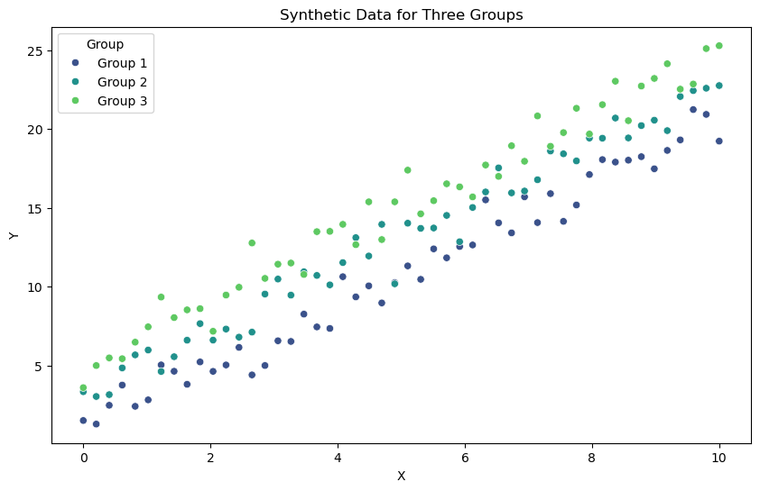
# Visualize the data
plt.figure(figsize=(10, 6))
sns.scatterplot(x=X, y=Y, hue=group_labels, palette='viridis')
plt.xlabel('X')
plt.ylabel('Y')
plt.title('Synthetic Data for Three Groups')
plt.legend(title='Group')
plt.show()
# Step 4: Define the Bayesian model
with pm.Model() as bayesian_model:
    # Shared slope for all groups
    slope = pm.Normal('slope', mu=0, sigma=10)

    # Intercepts for each group
    intercepts = pm.Normal('intercepts', mu=0, sigma=10, shape=3)

    # Noise standard deviation
    sigma = pm.HalfNormal('sigma', sigma=1)

    # Expected value of Y for each group
    # Use indexing to select the correct intercept for each data point based on its group
    mu = slope * X + intercepts[group_idx]

    # Likelihood (data generation process)
    Y_obs = pm.Normal('Y_obs', mu=mu, sigma=sigma, observed=Y)

    # Inference using Markov Chain Monte Carlo (MCMC)
    trace = pm.sample(1000, tune=1000, cores=2, target_accept=0.95)
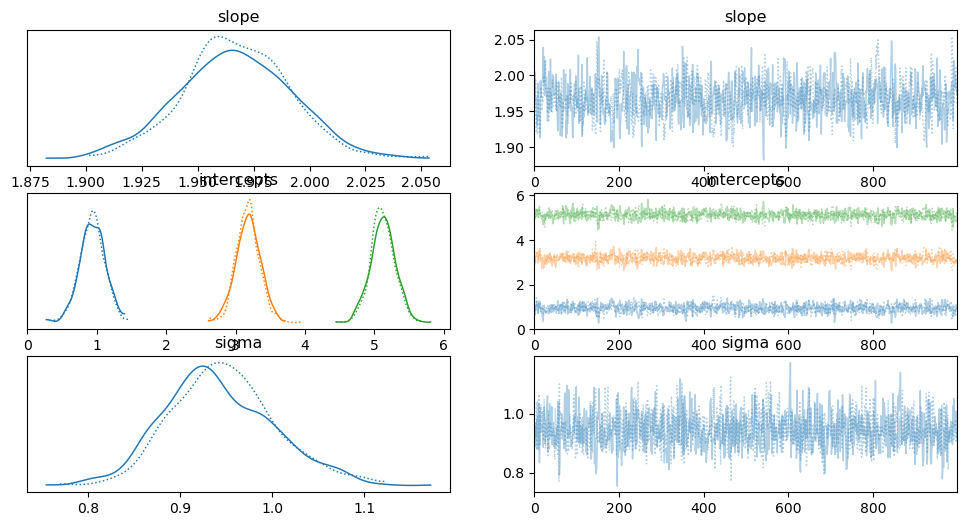
# Summarize the results
summary = pm.summary(trace)
print(summary)

# Plot the trace and posterior distributions for slope and intercepts
pm.traceplot(trace, var_names=['slope', 'intercepts', 'sigma'])
plt.show()
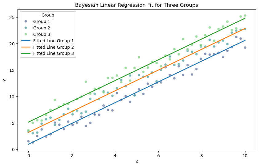
# Extract the mean posterior estimates for the slope and intercepts
mean_slope = np.mean(trace['slope'])
mean_intercepts = np.mean(trace['intercepts'], axis=0)

# Plot the data points
plt.figure(figsize=(10, 6))
sns.scatterplot(x=X, y=Y, hue=group_labels, palette='viridis', alpha=0.6)

# Plot the fitted lines for each group
x_vals = np.linspace(0, 10, 100)
for idx, intercept in enumerate(mean_intercepts):
    y_vals = mean_slope * x_vals + intercept
    plt.plot(x_vals, y_vals, label=f'Fitted Line Group {idx+1}', linewidth=2)

# Add labels and legend
plt.xlabel('X')
plt.ylabel('Y')
plt.title('Bayesian Linear Regression Fit for Three Groups')
plt.legend(title='Group')
plt.show()
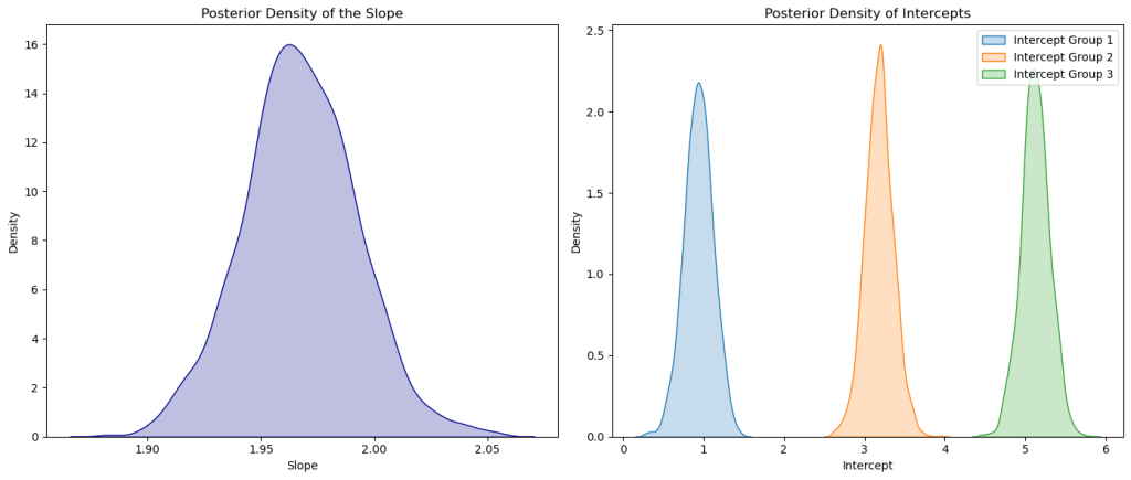
# Plot the posterior density for the slope
plt.figure(figsize=(14, 6))

plt.subplot(1, 2, 1)
sns.kdeplot(trace['slope'], color='darkblue', shade=True)
plt.title('Posterior Density of the Slope')
plt.xlabel('Slope')
plt.ylabel('Density')

# Plot the posterior densities for the intercepts of each group
plt.subplot(1, 2, 2)
for i in range(3):
    sns.kdeplot(trace['intercepts'][:, i], label=f'Intercept Group {i+1}', shade=True)
plt.title('Posterior Density of Intercepts')
plt.xlabel('Intercept')
plt.ylabel('Density')
plt.legend()

plt.tight_layout()
plt.show()